How to Use the FILTER Function in Excel?
The FILTER function allows you to extract specific data from a table based on given criteria.
Related reading
Excel Keyboard Shortcuts – Workbooks & Worksheets
These keyboard shortcuts help you manage workbooks and worksheets efficiently, giving quick access to common tasks in Microsoft Excel.
Comparison operators are used in Excel formulas to compare two values, and the result is either TRUE or FALSE. They are essential for creating logical tests within functions like IF.
➤ How to Use the FILTER Function
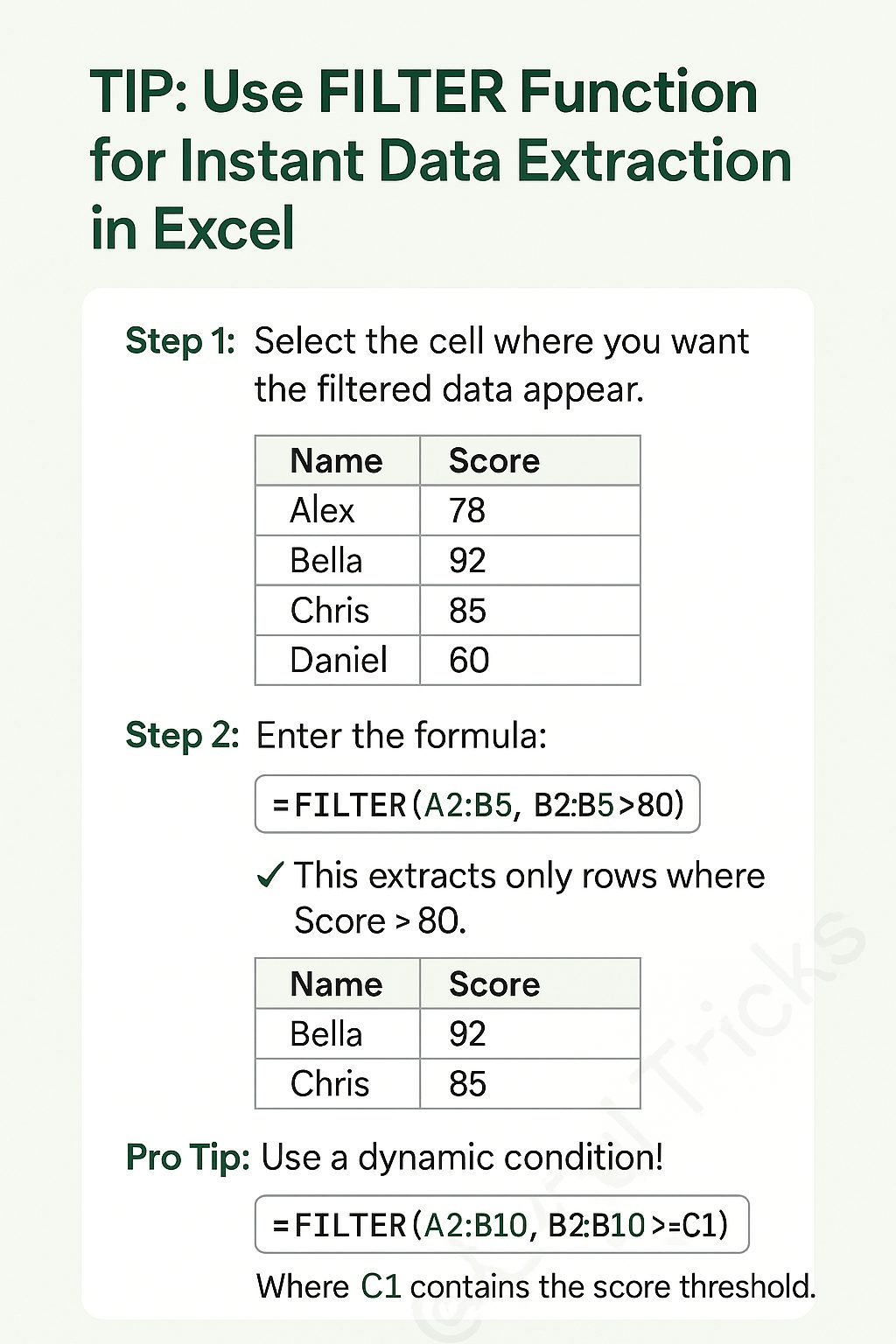
- Select the cell where the filtered data should appear.
- Enter the formula:
=FILTER(range, criteria)
➤ Example
Using the formula =FILTER(A2:B5, B2:B5>80) on a table with names and scores extracts only the rows where the score is greater than 80.
➤ Key Information
- Function: FILTER
- Purpose: Extract rows from a range of data that meet a specific condition.
- Formula Syntax:
=FILTER(array, include, [if_empty])
💡 Pro Tip
The criteria can be dynamic by referencing a cell. For example,
=FILTER(A2:B10, B2:B10 >= C1) filters the data based on a score threshold entered in cell C1.